Calibration of DSLR cameras
Contents
Calibration of DSLR cameras#
Absolute photometry#
For the absolute calibration of our system (telescope + filter + camera or DSLR + telescope or lens) we need to observe standar stars (stars whose magnitudes are known in the same system. These auxiliary observations are used as reference for the absolute calibration.
The observations from the ground are affected by the absortion of the earth atmosphere. This effect depends on the wavelength of the photons and it is different from night to night. The absolute photometry method rely in the observations during a clear and estable night when we can expect that the absortion is constant. The nights with this good astronomical conditions are called photometric nights.
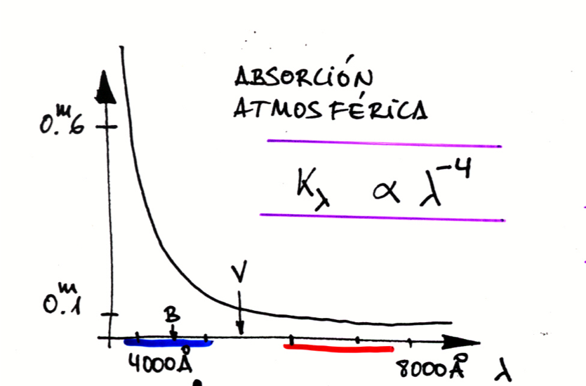
Fig. 10 La absorción atmosférica en el visible depende fuertemente de la longitud de onda.#
Basic equations#
The observed magnitude of a celestial object is obtained from the total flux measured (in counts/s or ADUs/s , analog to digital units)
where
\(C_{\lambda}\) is the instrumental constant or zero point
\(m_{\lambda}\) is the observed magnitude
\(F_{\lambda}\) is the net flux, i.e. corrected from sky brightness) in units of c/s.
The instrumental constants (or zero points) are system parameters different for every band as they depends on the spectral transmission of the filters, mirror reflectivity, aperture of the optical system, quantum efficiency of the detector etc. They do not change from one night to the next one during the observation campaign. But they are determined every time (for instance in a new campaign) since the change in the optics transmission or reflectivity of the mirrors etc. can change the overall sensitivity of the system.
The flux measured at ground for a celestial body is lower then the flux at the top of the atmosphere. The amount of extinction depends on the atmosphere transparency and the length of atmosphere that the light travel in the atmosphere. For instance this optical path is higher for observations near the horizon.
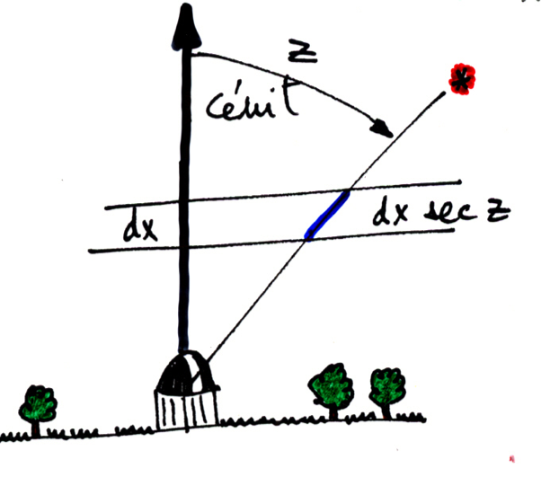
Fig. 11 The atmospheric extinction depends on the optical path that the light travels to reach the ground.#
donde
\(F_{\lambda}\) observed flux
\(F_{\lambda}^0\) flux at the top of the atmosphere
\(K_{\lambda}\) extinction coeficient
\(z\) zenith angle
\(\sec(z)\) airmass
\(m_{\lambda}\) observed magnitude
\(m_{\lambda}^0\) extinction corrected magnitude or magnitude on top of the atmosphere
To determine the zero points and the extinction coeficients we must observe standar stars at different airmasses during photometric nights (clear, estable, transparent) when we expect low extinction coefficients.
By combining the equations, the fundamental equation arises:
The graph \(m_{\lambda}^0 + 2.5 \times \log_{10} F_{\lambda}(\text{c/s})\) versus \(\sec(z)\), with the observations. The points can be fitted with a line (‘Bouger line’) where the intersection with the Y-axis is \(C_{\lambda}\) and the slope \(-K_{\lambda}\). The quality of the fit is a sign of the astronomical quality of the night. The dispersion of the observations is a sign of variable extinction. Nights with good transparency has lower slope in the fit, i.e. low calues of the extinction coeficient.
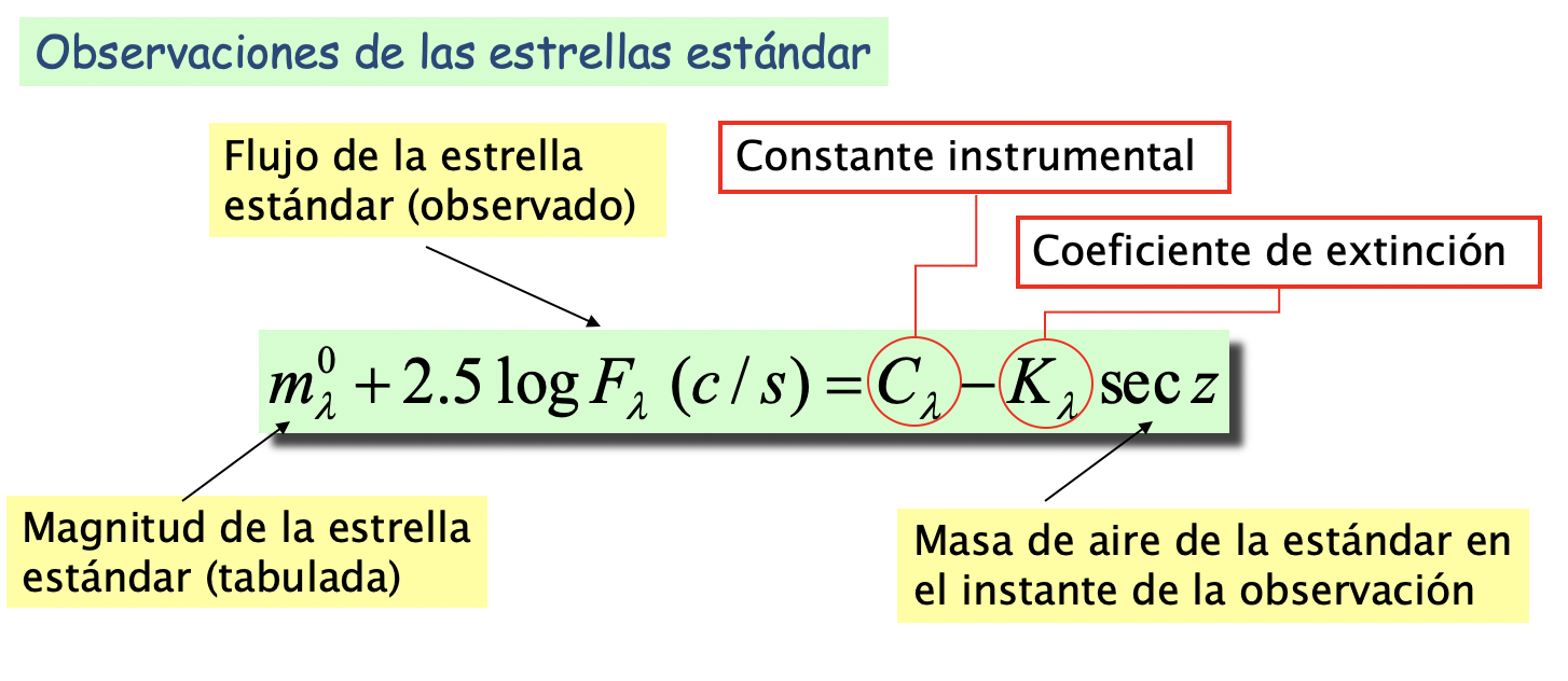
Fig. 12 TODO: repeat schematics in english#
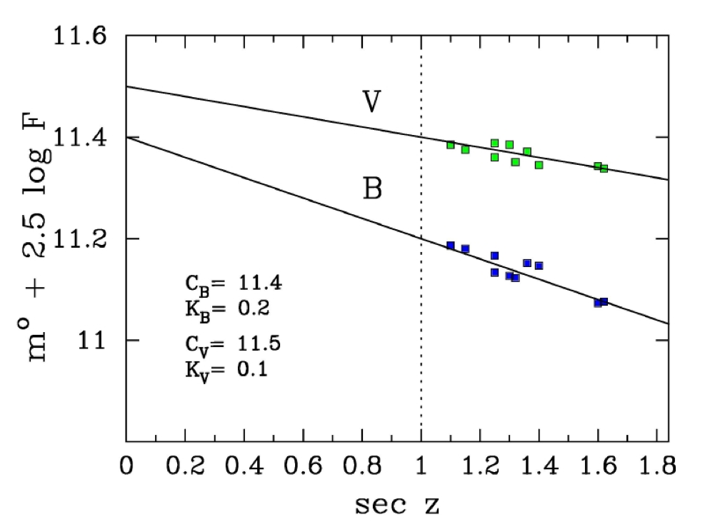
Fig. 13 Example of observations in Johnson-Cousins \(B\) and \(V\) bands. Note the higher slope in \(B\) band as expected.#
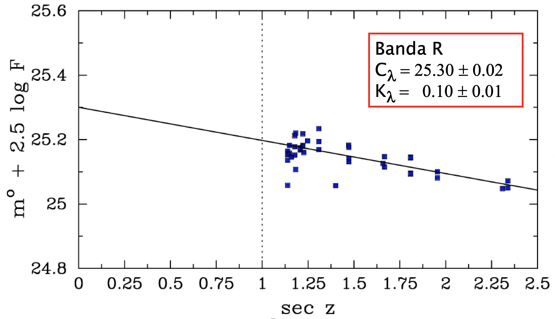
Fig. 14 The dispersion of the points is a measure of the photometric quality of the night and allow us to determine the accuracy of the photometry.#
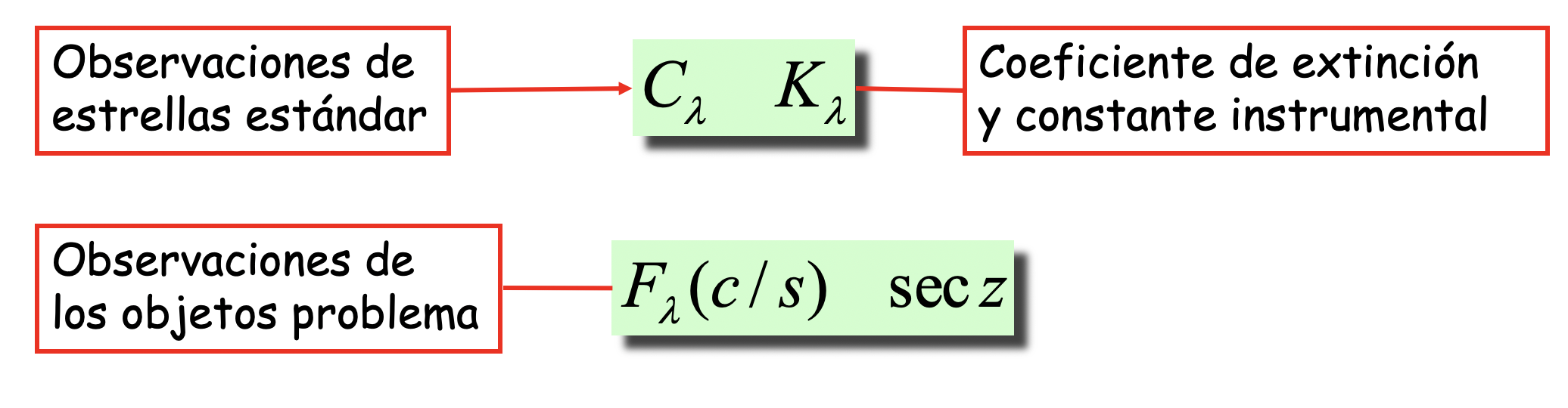
Fig. 15 TODO: repeat schematics in english Las observaciones auxiliares de estrellas estándar nos permiten determinar las constantes instrumentales y el coeficiente de extinción de esa noche.#
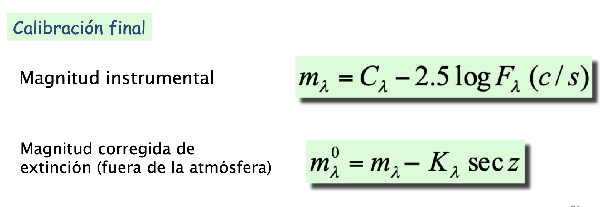
Fig. 16 TODO: repeat schematics in english Con el flujo en c/s de nuestro objeto de interés podemos determinar la magnitud instrumental y luego corregirla del efecto de la atmósfera gracias a que hemos determinado previamente \(C_\lambda\) y \(K_\lambda\).#
Astronomical calibration of DSLRs#
With an RGB photometric system which provide millions of stars whose magnitude is tabulated it is possible to calibrate the camera system using the method of ‘Astronomical Absolute Photometry’.
The zero point or instrumental constant for each band is the only parameter needed to convert from observed fluxes (ADUs/s) into physical units (magnitudes). It should be noted that the zero point do not depend on the atmosphere conditions. That means that we can calibrate the camera one photometric night an use this calibration for other nights.
Calibration of a Nikon D3#
Observations#
This example shows the calibration of a Nikon D3 camera with 50mm lens at f/1.8 ISO1600 exposure 3s with observations at Berlin coor=[52.457941, 13.310668]. date=’2013/10/24 23:13:33’ #UT (local time ‘2013/10/25 01:13:33’)
picture    obstime    model    focal    fnumber    iso    exposure
_DSC5223    2013-10-24 23:12:53    NIKON D3    50    1.8    1600    3
_DSC5224    2013-10-24 23:13:33    NIKON D3    50    1.8    1600    3
_DSC5225    2013-10-24 23:14:02    NIKON D3    50    1.8    1600    3
_DSC5226    2013-10-24 23:14:20    NIKON D3    50    1.8    1600    3
_DSC5227    2013-10-24 23:14:48    NIKON D3    50    1.8    1600    3
_DSC5228    2013-10-24 23:15:07    NIKON D3    50    1.8    1600    3
_DSC5229    2013-10-24 23:15:33    NIKON D3    50    1.8    1600    3
Defocuss#
After the first focussed picture (DSC5223 .NEF) it was decided to defocuss the remain shots to get star images with a wider area in order to perform a better photometry.
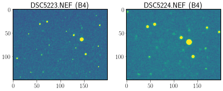
Fig. 17 Same field of stars with two different focus adjustement. The image at right shows the slightly out of focus observations to better sampling the star images.#
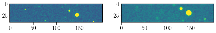
Fig. 18 Same as Fig. 17 showing two bright stars used for comparison.#
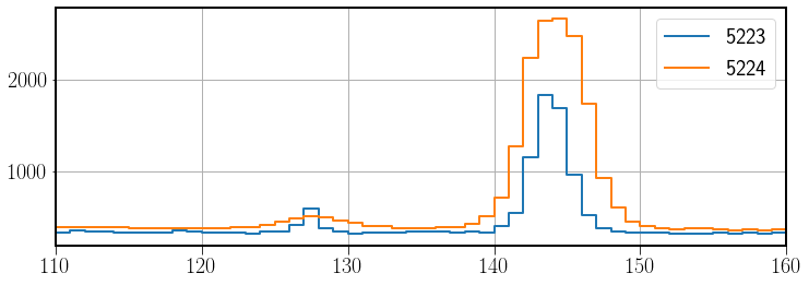
Fig. 19 Cross along the star images to show the widening when picture is defocused.#
It should be noted that distributing the photons arriving from the stars in a wider area disminished the signal to noise ratio of the observation. On the other hand, bright stars whose focussed images would saturate could be measured when the light is smeared.
RGB demosaicing#
The RGB images should be extracted from the RAW pictures.
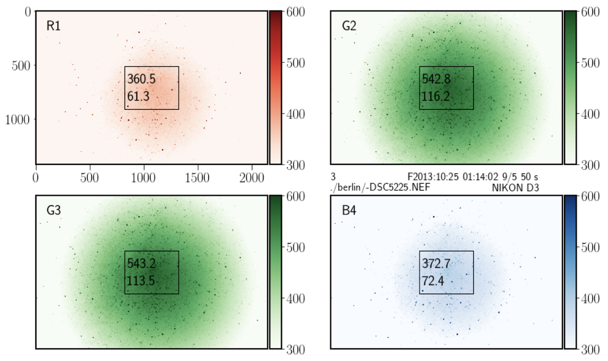
Fig. 20 The picture DSC5225.NEF after decomposition in the 4 channels RGGB. The vignetting effect is apparent.#
The resulting images are labelled R1, G2, G3 and R4 indicating the color and the channel number. Green images G2 and G3 should be similar.
Vignetting#
There is a lost of light at the periphery of the pictures (optical vignetting) should be corrected. This effect is worse in low cost lenses and depends on the diafragm or aperture (f/number). There ara several methods to obtain these ‘FLATSs’ images used to correct the observations. Without any correction the fluxes of stars imaged at peripheral positions are lower and not comparable to those stars on the optical axis, i.e. in the center of the image.
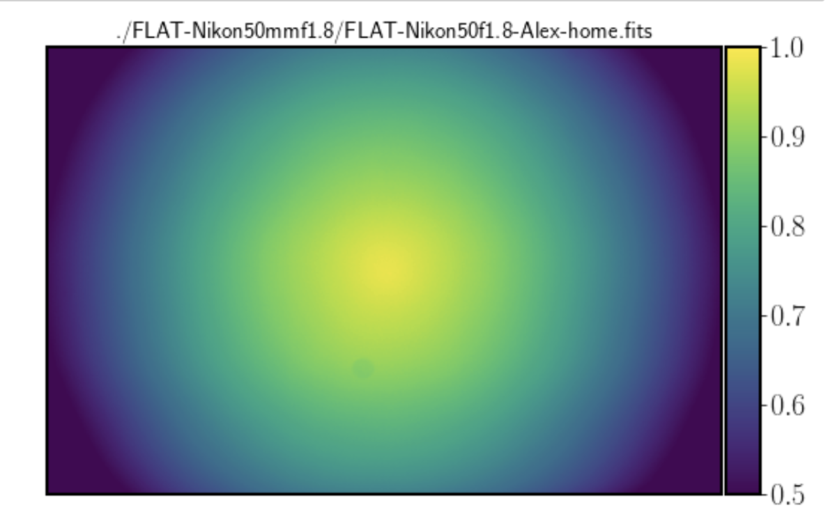
Fig. 21 The image of the flat obtained with a flat screen that model the vignetting effect. Note the drop in light in the corners of the image.#
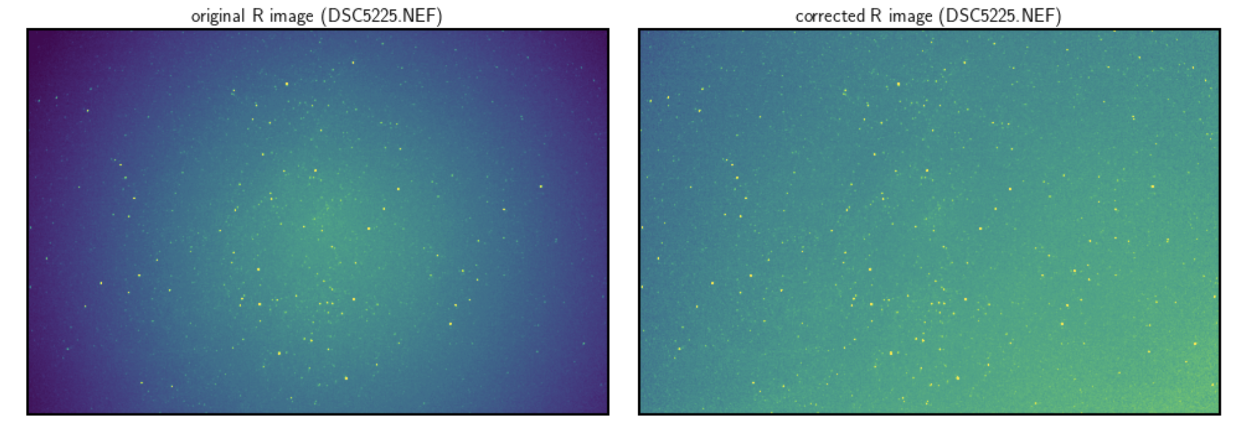
Fig. 22 The original and corrected image (at right) after division by the normalized flat image.#
Astrometry#
Before measuring the star fluxes we must determine to which star correspond each star image in the picture. This step implies to perform astrometry to determine the transform form pixels in the picture to coordinates in the sky.
With Astrometry.net we can get the WCS descriptor of the astrometric calibration. For example for DSC5224 we detect 161 sources (using find_peaks in python) and sent the 80 brightest sources to Astrometry.net that determines the pointing, field of view, and the scale of the picture.
CRVAL1  =        14.3972939394    / RA  of reference point
CRVAL2  =        61.6447899891    / DEC of reference point
CRPIX1  =        1176.33333333     / X reference pixel
CRPIX2  =        685.666666667     / Y reference pixel
CUNIT1  = 'deg     '                       / X pixel scale units
CUNIT2  = 'deg     '                       / Y pixel scale units
CD1_1   =     0.00881987432631  / Transformation matrix
CD1_2   =     -0.0167280233886  / no comment
CD2_1   =      0.0167278788786  / no comment
CD2_2   =     0.00887402089068 / no comment
IMAGEW  =                 2144         / Image width,  in pixels.
IMAGEH  =                 1422          / Image height, in pixels.
Number of WCS axes: 2
CTYPE : 'RA---TAN-SIP'  'DEC--TAN-SIP'
CRVAL : 14.3972939394  61.6447899891
CRPIX : 1176.33333333  685.666666667
CD1_1 CD1_2  : 0.00881987432631  -0.0167280233886
CD2_1 CD2_2  : 0.0167278788786  0.00887402089068
NAXIS : 0  0
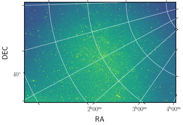
Fig. 23 Picture DSC5224 (channel G) after performing the astrometry.#
Photometry#
We intend to measure the fluxes (in each channel) of the star images in the field of view that are tabulated in the catalogue of RGB standard stars. The first step is to determine which star are the standard and their XY position.
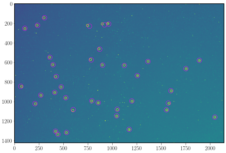
Fig. 24 The RGB stars of this image are detected in the expected positions determined by the astrometry.#
After creating a table with stars positions X,Y, name, flux in each channel etc. we can prepare the graph to fit the Bouger line and determine the photometry parameters.
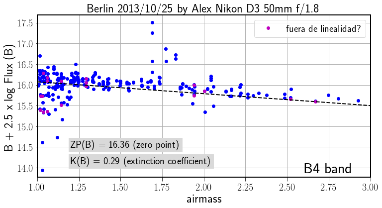
Fig. 25 Bouger fit for B band.#
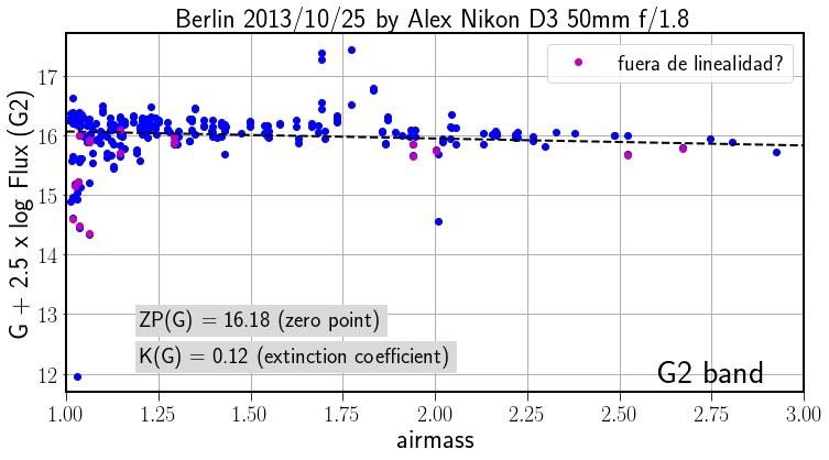
Fig. 26 Bouger fit for G band.#
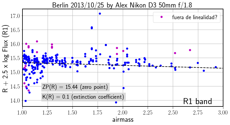
Fig. 27 Bouger fit for R band.#
Sky brightness#
To determine sky brightness we need to know the plate scale, i.e. the transformation of pixel size in mm to pixel projected in the sky (arcsec). The WCS astrometric transformation provide: 0.0189 deg/pixel or 68.08 arcsec/pixel. We can determine this values using the size of the pixel and the focal of the camera:
# Nikon D3
Effective Megapixels:    12.1
Sensor Format:    35mm
Sensor size:    860.4mm2 (36.00mm x 23.90mm)
Approximate Pixel Pitch:    8.46 microns

f = 50                          # mm
P = 206265 / 50         # arcsec/mm
pp = P * 8.46 / 1000   # arcsec
34.90 arcsec/pixel
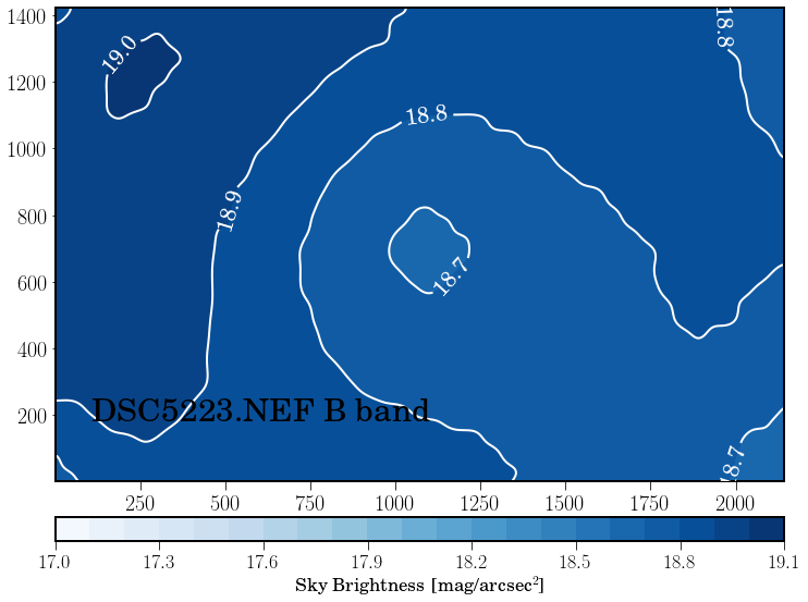
Fig. 28 Sky brightness in B< band.#
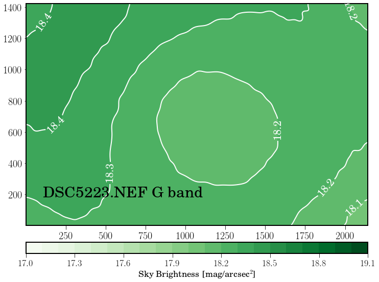
Fig. 29 Sky brightness in G band.#
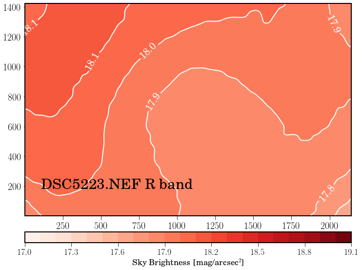
Fig. 30 Sky brightness in R band.#