Astronomical spectroscopy calibration
Contents
Astronomical spectroscopy calibration#
Motivation#
During the last years the number of amateur astronomers interested in spectroscopy is increasing. For a first look to spectrographs and methods browse Christian Buil home page
Besides profesional astronomical software, there are user friendly software to analyse spectra taken with the simple spectrographs that the amateur are using. Amateur astronomers can extract the monodimensional spectra, calibrate in wavelength, etc.
To derive the spectral response curve of the spectrograph we can compare one star spectrum observation with the calibrated spectrum published in a spectrum atlas. The observed spectrum is affected from atmospheric extinction and we can not compare directly this spectrum with the tabulated spectrum of the star which is corrected, i.e. is the spectrum that we would observe ‘outside the atmosphere’.
We describe an observational method to derive the spectral response curve of the system after correcting from atmospheric extinction. Several observations at different airmass are used to derive atmospheric extinction.
Modelling the observation of a star with a spectrograph#
To understand the method let model the spectrum of a star observed from ground with a spectrograph fitted to a telescope. Let us use Vega as the standard star. The tabulated spectrum of Vega can be found in a star atlas and represent the amount of flux per unit wavelength.
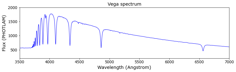
Fig. 120 Spectrum of Vega used for the modelling.#
Atmospheric extinction#
The amount of extinction depends on the atmosphere conditions \(K_\lambda\) (extinction coefficient) that is constant for a photometric night but different from night to night, and the optical path of the light in the atmosphere \(secz\) (airmass). The extinction coefficient can be derived, for example, from observations of one star at different altitudes during the night. For the modelling let us assume that the extinction at 5500 Angstrom is \(K_\lambda = 0.3\) and that the dependence with wavelength is \( K_\lambda = \lambda^{-4}\).
Note
You can find in Note technique “Le calcul de la transmission spectrale atmosphérique: application à la surveillance de l’activité Be d’étoiles faibles” (C. Buil - 09/02/2009) a more detailed model of the dependence of the extinction.
The extinction \(K_\lambda\) is given as magnitudes per airmass. The amount of extinction depends on the airmass \(secz\). The observed spectrum from ground \(F^{obs}_\lambda\) is related to the ‘out of the atmosphere’ spectrum \(F^{o}_\lambda\) as
where \(S_\lambda\) is the spectral response.
In what follows let us assume for the modelling that the spectral response is constant \(S_\lambda = 1 \) to appreciate the effects of extinction at different air masses.

Fig. 121 Variation of extinction with wavelength. We have modelled K=0.3 for 5500 Angstrom.#
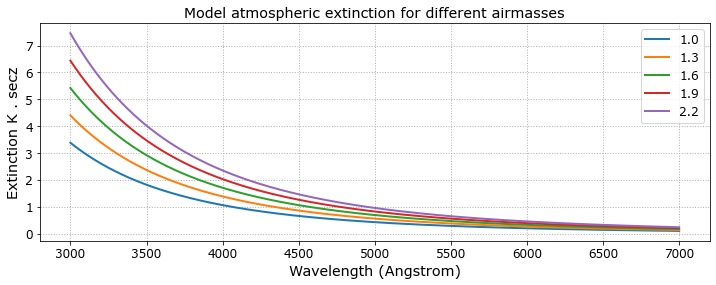
Fig. 122 Amount of extinction for different airmasses.#
Applying atmospheric extinction#
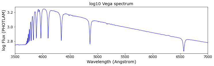
Fig. 123 Model Vega log spectrum.#

Fig. 124 Model observed Vega log spectrum for different airmasses.#
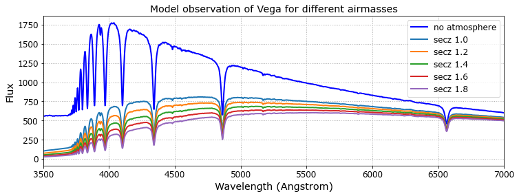
Fig. 125 Model observed Vega spectrum for different airmasses.#
Deriving \(K_\lambda\) and \(S_\lambda\) from observations#
Calibration night#
Let observe the same star at two or more different air masses. For calibration it is recommended to use a hot star (O,B,A star) with enough signal in the blue region of the spectrum where the atmospheric absorption is higher.
The resulting observed spectra for these observations should be:
where \(F^{o}_\lambda\) ; \(S_\lambda\) and \(K_\lambda\) are the same in both equations. Comparing the spectra,
and we can determine \(K_\lambda\) for this night.
\(S_\lambda\) is obtained from one of the spectra after \(K_\lambda\) is known,
The response curve \(S_\lambda\) obtained can be used for any other night if the settings of the instrument are maintained.
Science night#
During an observation to obtain the spectrum of a target star we need to determine the extinction curve to correct from the atmosphere effects.
One simple method is to observe our target star at two different air masses. By comparing them we derive the extinction. The spectrum of the target star is corrected from response curve and then from extinction.
Usually the extinction is considered constant along a photometric night. We can derive it by comparing the spectrum of any spectrophotometric standard star (after correction of the response curve) with the tabulated spectrum. This extinction curve is valid for all the observation of this night. again: The spectrum of the target star is corrected from response curve and then from the extinction determined by this method. Please note that only one extra observation of a standard star is needed for calibration.