RGB photometry examples
Contents
RGB photometry examples#
Differential photometry#
Series of observations with the same equipment and settings can be compared to determine photometric evolution. This is useful to follow the light curve of astronomical objects.
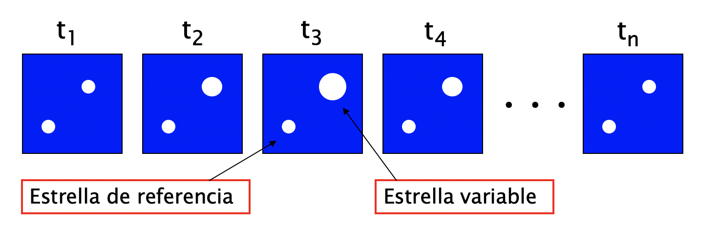
Fig. 51 Series of pictures with problem star and the star used as reference.#
To understand the differential photometry method let show the main equations. The instrumental magnitude \(m_\lambda\) of a star is determined as,
where \(C_\lambda\) is the instrumental constant or zero point, \(F_\lambda\) is the observed flux (counts/s), K_\lambda is the extinction coefficient at the observing time and \(secz\) is the airmass (\(z\) cenital angle). The amount of extinction depends on the extinction coefficient and the length of the path of the light into the atmosphere.
For an observation with a panoramic detector (image observation) the images of the problem star (for instance a variable star) and the reference star (or stars) are obtained at the same time with the same equipment and settings, at the same position in the sky.
In this case \(C_\lambda\), \(K_\lambda\) and \(secz\) is equal in the two equations and,
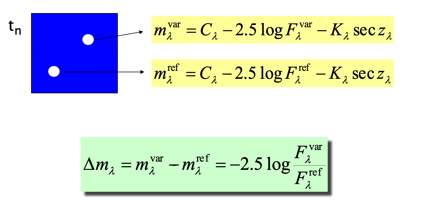
Fig. 52 Equations for the star fluxes and magnitudes.#
We are using the \(\lambda\) subscript to indicate that the flux, extinction coefficient and instrumental constant depends on the wavelength. For a photometric band as \(B\) the equations is,
and we can derive the magnitude of the variable star as,
When there are several reference stars in the Field of View (FoV) of the image obtained during the observation one can use all of then to determine the magnitude of the variable star.
where \((C_B - K_B \; secz)\) in equation (*) is determined with all the reference stars in the FoV of the image.
Using differential photometry is easy as we do not need very clear and stable ‘photometric nights’. Repeating the observations at different epochs we can build the ‘light curve’ of the variable star.
Example 1: SN2023bee RGB light curve#
The Type Ia supernova SN2023bee in NGC2708 was discovered on 2023-02-01.
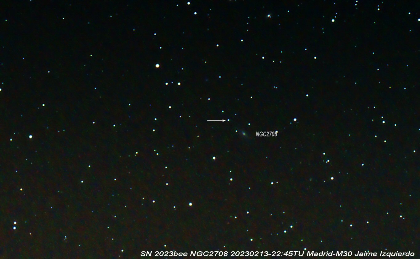
Fig. 53 SN2023bee in NGC2708 by Jaime Izquierdo from Madrid on 20230213 22:45TU using Takahashi 130 + DSLR PentaxK1. This is a composition of 40 shots taken without filter.#
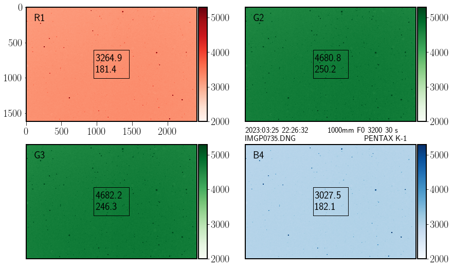
Fig. 54 After debayering one of the pictures of SN2023bee obtained by Jaime Izquierdo.#
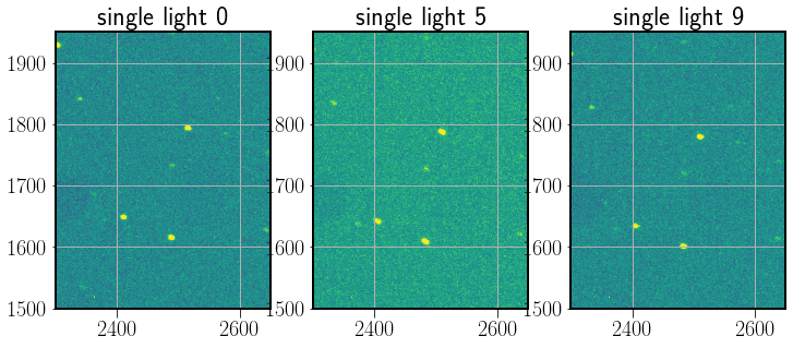
Fig. 55 There is a small displacement between individual pictures.#
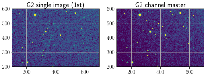
Fig. 56 After registering and combining the individual images.#
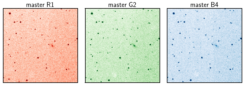
Fig. 57 The R, G, and B channels of the master images after the combination.#
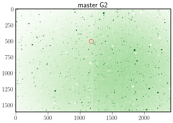
Fig. 58 One of the G channels of the master images after the combination. Complete image.#
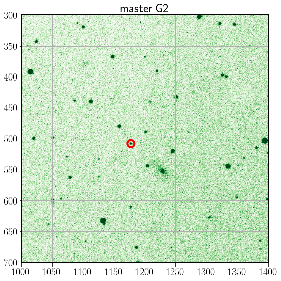
Fig. 59 One of the G channels of the master images after the combination. Crop image for detail view.#
Astrometry#
We are interested in perform the astrometry of the images to determine which standard stars are in the field of view. It is posible to upload to Astrometry.net a table with the sources positions (X,Y) in the image. This method is faster than uploading the whole image.
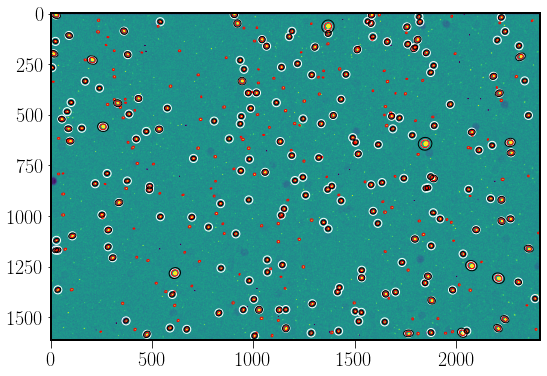
Fig. 60 Finding objects in the image to build a table of sources and positions X,Y.#
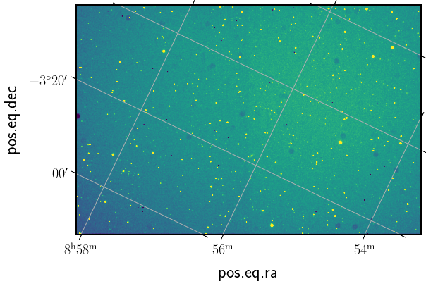
Fig. 61 Image (channel G2) after astrometry.#
In this example the pixel scale is 2.00909127, 2.00852395 arcsec/pixel
Photometry#
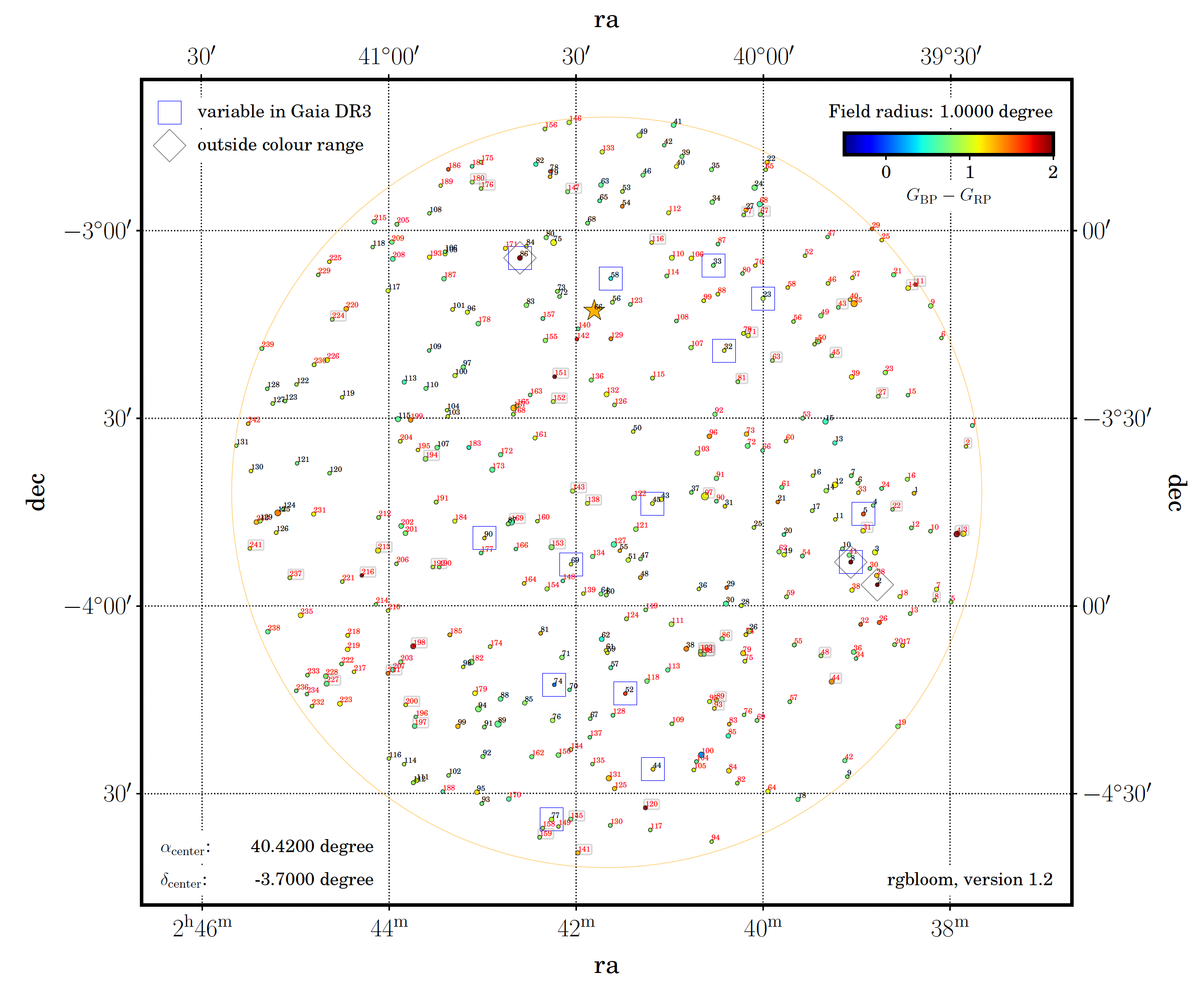
Fig. 62 Chart of RGB standard stars in the coordinates of the SN2023bee. For this search up to magnitude m=14 RGBloom has found 242 standard stars in a 1 degree radius around the supernova.#
The RGBloom software is a Python script that retrieves RGB magnitudes computed from low resolution spectra published in Gaia DR3, following the work described in Carrasco et al. (2023). These magnitudes are given in the standard system defined by Cardiel et al. (2021a).
After installing the open software, the command
rgbloom 40.42 -3.70 1 14
returns a chart and a catalog of standard stars,
number,source_id,ra,dec,RGB_B,RGB_G,RGB_R,errRGB_B,errRGB_G,errRGB_R,objtype,qlflag
       1, 2495417093223451904,  39.441520505,  -3.519326264, 13.0408, 12.8512, 12.7202,  0.0013,  0.0011,  0.0017,0,0
       2, 2495228943591313152,  39.458562077,  -3.575288465, 14.1979, 13.9068, 13.7532,  0.0049,  0.0057,  0.0216,0,1
       3, 2495116587246963072,  39.465498677,  -3.807688942, 10.6774, 10.2936,  9.9891,  0.0015,  0.0013,  0.0018,0,1

     241, 5185635284310164352,  41.371700175,  -3.847027674, 14.6271, 14.2388, 13.9169,  0.0021,  0.0016,  0.0022,0,1
     242, 5185699949337739648,  41.375780195,  -3.514606896, 14.6113, 14.2008, 13.8180,  0.0025,  0.0017,  0.0023,0,0
With the astrometry done we can convert equatorial coordinates (ra,dec) of the standard stars to X,Y positions in the image.
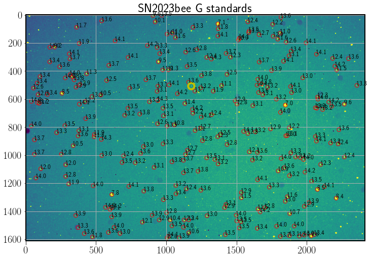
Fig. 63 RGB standards found the image. A yellow circle marks the supernova.#
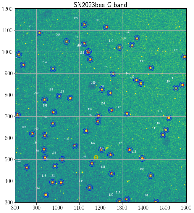
Fig. 64 Photometry of the RGB standards found the image. A yellow circle marks the supernova. The image is cropped for detailed view.#
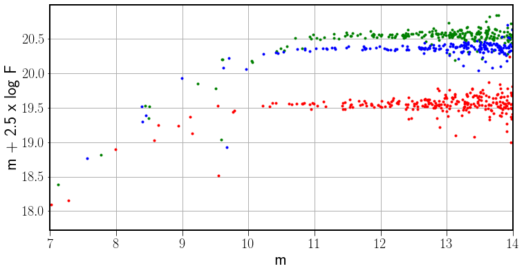
Fig. 65 The \(m + 2.5 \times log_{10}\; F\) graph shows the saturation for stars brighter than magnitude 11.#
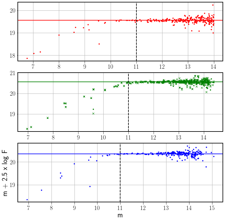
Fig. 66 Final R, G and B \(m + 2.5 \times log_{10}\; F\) for each of the channels. The lines show the mean value for stars fainter than m=11. For the G channels the star magnitude symbol is a point for G2 and a cross for G3.#
We obtain the zero point = \(m + 2.5 \times log_{10}\; F\) for this observation
\(ZP_{R1} = 19.56 \;\; \;\; ZP_{G2} = 20.557 \;\;\;\; ZP_{G3} = 20.556 \;\; \;\; ZP_{B4} = 20.36\)
After measuring the supernova fluxes for the 4 channels,
\(F_{R1} = 101.4 \;\; \;\; F_{G2} = 222.9 \;\;\;\; F_{G3} = 220.8 \;\; \;\; F_{B4} = 127.6\) [counts/s]
We can obtain the RGB magnitude of the supernova, \(R = ZP_{R} - 2.5 \times log_{10}\; F_{R}\)
\(R1 = 14.547 \;\; \;\; G2 = 14.687 \;\; \;\; G3 = 14.695 \;\; \;\; B4 = 15.098\)
Jaime Izquierdo from Madrid Takahashi + Pentax K1
30s exposures  3200 ISO
2023-03-25T22:26:32 UTC  R=14.55  G=14.69  B=15.10 JD=2460029.43509259
Light curve#
With observations taken at different nights we can build the light curve. For this example we have observations taken with different equipment:
Jaime Izquierdo  Madrid Takahashi + Pentax K1
Jaime Izquierdo  Madrid Takahashi + QHY5III290C
David Ibarra     Ager   150mm f7 + ZWO ASI533MC
David Ibarra     San Vicente de Raspeig   150mm f7 + ZWO ASI533MC
Sergio Vilanova Puig de Santa María  300mm Meade 850 Canon EOS 250D
The table of results
2459992.47006944, 13.28, 13.14, 13.1
2460000.42910880, 13.40, 13.31, 13.29
2460008.42910880, 13.61, 13.85, 13.74
2459993.52986111, 13.30, 13.15, 13.07
2460004.48788194, 13.68, 13.50, 13.45
2460004.44262732, 13.65, 13.54, 13.49
2459998.44709491, 13.12, 13.10, 13.11
2460000.49375000, 13.20, 13.18, 13.18
2460014.45504630, 13.59, 11.04, 14.42
2460014.44971065, 12.89, 14.06, 14.26
2460029.43509259, 14.55, 14.69, 15.10
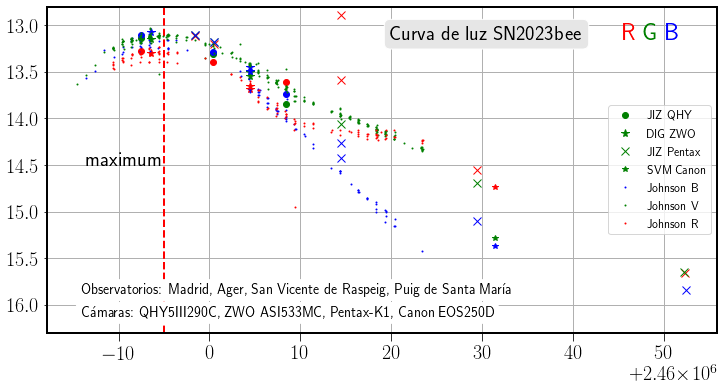
Fig. 67 Light curve using RGB photometry with observations by Jaime Izquierdo, David Ibarra and Sergio Vilanova. Small dots are Johnson B, V and R measures by Agrupación Astronómica de Madrid (AAM) observers.#